

Current Sensing Architectures in 100kHz–200kHz GaN Servo Inverters: In-Line Shunts, Low-Side Limits, and Isolated Magnetic ICs in Robotics Procurement
Compare GaN servo current sensing: in-line shunts, low-side limits and isolated magnetic ICs. Use timing examples and an 8-point RFQ checklist for OEM sourcing.
For 24V–60V GaN servo drives at 100 kHz–200 kHz PWM, select current sensing by usable acquisition time, switching-transient recovery, measurement error, and fault response. Low-side shunts can be economical when the required switching states leave enough sampling time. In-line shunts remove that conduction-state restriction but still require quiet sampling intervals. Isolated magnetic ICs add an isolation barrier, with device-specific bandwidth, conductor loss, and protection latency.
Executive Summary (TL;DR)
- At 100 kHz and 90% phase duty, total low-side conduction is 1 µs per period; at 200 kHz it is 0.5 µs. The usable contiguous window depends on PWM sequencing and dead-time.
- In-line sensing measures phase current through both switching states, but ADC acquisition must avoid common-mode transient recovery. Enhanced PWM rejection is not blanket approval for 200 kHz operation.
- Units matter: 500 V/µs equals 0.5 V/ns. Compare datasheet test edges with the measured board edge rather than treating AC CMRR or bandwidth as a slew-rate guarantee.
- An isolation barrier does not eliminate capacitive coupling, magnetic interference, conductor heating, or delay. Verify the exact sensor variant and its complete fault-to-gate-off path.
- Use the 8-point RFQ checklist below to request waveforms, error budgets, thermal evidence, and independent hardware overcurrent protection.
Published and reviewed: November 1, 2026. Scope: Global robotics OEMs, automation integrators, and motion-control engineers comparing current sensing in 24V–60V DC GaN servo inverters. The examples use a nominal 48V bus and PMSM/BLDC phase currents. Battery charge voltage, regenerative overshoot, phase-node undershoot, motor inductance, and cable length must be specified separately.
Evidence and calculation limits: This is a datasheet-based selection framework with reproducible calculations, not a measured comparison of production drives. Timing and parasitic values below are explicit assumptions. No component listing establishes 200 kHz suitability, certified isolation, functional safety, or system stability. See the official sources and their boundaries.
Start with the 24V GaN FOC timing tool or 24V low-voltage GaN servo module guide. These are planning resources; confirm your actual voltage and sensing requirements with the GAN Servo engineering team.
1. Why Higher PWM Frequency Tightens the Current-Sensing Budget
GaN devices can reduce switching losses in a suitable design; switching loss, output-capacitance loss, conduction loss, and thermal limits remain. Increasing PWM from an illustrative 20 kHz to 100 kHz–200 kHz shortens the period from 50 µs to 10 µs–5 µs. It can reduce current ripple for the same voltage, inductance, and modulation, but does not by itself establish higher closed-loop bandwidth or remove filtering requirements.
Two separate constraints drive procurement decisions:
- Available time: Low-side sensing needs an appropriate conducting state long enough for edge blanking, amplifier recovery, and ADC acquisition. The limiting state depends on the number of shunts, PWM sector, and sampling strategy.
- Transient recovery: In-line sensing sees the switching phase voltage. Determine the actual voltage excursion and rise/fall time; do not infer slew rate from the GaN label. A 48V transition over 2 ns–5 ns averages 24 V/ns–9.6 V/ns. Faster edges and ringing require separate measurements.
PWM carrier frequency, ADC sample rate, FOC update rate, motor electrical frequency, and closed-loop bandwidth are different quantities. Require suppliers to report each one.
2. Low-Side Shunts: Calculate the Available Window
For phase duty D_x and PWM frequency f_sw, the ideal total low-side commanded time per period is:
t_low_total = (1 - D_x) / f_swHere D_x is one phase's high-side duty, not the overall SVPWM modulation index or the fraction of available motor speed. A center-aligned implementation may place this time across a period boundary; other sequences may split it. Simultaneous two-phase measurements can have a shorter shared interval. Use the actual timer states to find the contiguous acquisition window.
For a conservative sequential timing example:
t_required = t_dead + t_ring + t_settle + t_acquireUse measured common-mode recovery to the required error band, not small-signal bandwidth alone. Some delays overlap in real hardware; avoid double-counting when using measured recovery. A 0.1% settling criterion is approximately one 10-bit full-scale LSB and about four 12-bit LSBs, not 12-bit accuracy.
The following are assumed timing budgets, not measurements or typical values for all silicon/GaN drives:
Case A: 20 kHz, phase duty D_x = 0.90
Total low-side time = 0.10 × 50,000 ns = 5,000 ns
Assumed delays = 250 + 400 + 800 + 250 = 1,700 ns
Upper-bound margin = 5,000 - 1,700 = +3,300 ns

Case B: 100 kHz, phase duty D_x = 0.90
Total low-side time = 0.10 × 10,000 ns = 1,000 ns
Assumed delays = 25 + 200 + 600 + 200 = 1,025 ns
Upper-bound margin = 1,000 - 1,025 = -25 ns

Case C: 200 kHz, phase duty D_x = 0.90, same assumed delays
Total low-side time = 0.10 × 5,000 ns = 500 ns
Upper-bound margin = 500 - 1,025 = -525 ns
A negative margin rejects this particular acquisition budget. A positive total-time margin still needs confirmation against the contiguous switching-state window. Under the simplified model, D_max = 1 - f_sw × t_required: 89.75% at 100 kHz and 79.5% at 200 kHz for the assumed 1.025 µs requirement, before extra margin.
Faster acquisition, different sampling states, pulse shifts, reconstruction, or duty limiting may recover operating range. Their torque-ripple and acoustic effects must be measured; low-side sensing is not automatically unsuitable above a fixed duty. Fault currents may bypass a low-side shunt depending on fault location and grounding, so request a fault-path analysis.
3. In-Line Phase Shunts: Distinguish CMRR, Recovery, and Slew Rate
An in-line shunt sits between the inverter phase node and motor winding. Phase current passes through it during both high-side and low-side conduction, removing the need to wait for a low-side state. The amplifier output can still be disturbed around PWM edges, and ADC sampling must wait for recovery. Shunt placement alone does not guarantee full modulation range, fault coverage, or sub-microsecond shutdown.
A Reproducible Parasitic-Coupling Example
Assume a 48V bus, a 1 ns 10%–90% transition, and an effective 2 pF coupling capacitance:
dv/dt = 0.8 × 48 V / 1 ns = 38.4 V/ns = 38,400 V/µs
I_displacement = C × dv/dt
               = 2 × 10^-12 F × 38.4 × 10^9 V/s
               = 76.8 mA during the transition
This estimates current through the assumed coupling capacitance. It is not a measurement of current entering an amplifier pin or a differential error: the coupling path, input matching, impedance, and filtering determine the resulting disturbance. It cannot establish a universal saturation or recovery time.
What the Published Specifications Actually Support
The TI INA240 datasheet lists a −4V to 80V operating common-mode range and 93 dB AC CMRR at 50 kHz. The TI INA241x datasheet lists −5V to 110V operation, 1.1 MHz small-signal bandwidth, and support for switching frequencies up to 125 kHz. That does not approve INA241x for 200 kHz PWM.
The ADI MAX40056 datasheet lists 500 ns PWM-edge recovery for a 500 V/µs edge. 500 V/µs = 0.5 V/ns, substantially slower than the assumed 38.4 V/ns example. A quoted recovery time at one edge rate cannot be transferred to another without evidence.
AC CMRR is a frequency-dependent rejection measurement; PWM recovery is a time-domain response to a stated edge. Isolation CMTI is another test with its own conditions. Specify the required residual output error at the intended ADC instant, actual positive/negative common-mode extremes, gain, input filters, supply, and temperature.
4. Current-Sensing Architecture and Timing Diagram
The diagram compares placements and reproduces Case B. It is an illustrative circuit and timing budget, not an approved schematic or oscilloscope capture. Scroll horizontally on small screens for readable labels.
Figure 1: Alternative shunt placements and the assumed Case B timing budget. In-line sensing still needs PWM-transient recovery; low-side suitability depends on the actual acquisition window.
5. Architectural Comparison Matrix
These are selection trade-offs, not guaranteed performance or quoted BOM prices. The cited magnetic example is Hall-based; do not transfer its specifications to GMR or other magnetic ICs.
| Selection metric | In-line shunt + PWM-rejection amplifier | Three low-side shunts | Isolated magnetic IC |
|---|---|---|---|
| Example / identity | INA240, INA241x, MAX40056; verify exact gain/variant | Shunts and suitable ground-referenced amplifiers | ACS37002 Hall example; qualify other Hall/GMR parts separately |
| Acquisition availability | Both conduction states; avoid edge recovery | Needs valid low-side states and reconstruction policy | Independent of low-side state; check output settling |
| PWM-frequency suitability | Device-specific; INA241x lists up to 125 kHz | Determine contiguous window at required duty and sector | Analog bandwidth alone does not approve a PWM frequency |
| Transient susceptibility | Common-mode range, undershoot, PWM recovery, filter mismatch | Ground bounce, ringing, and common-source inductance | Barrier capacitance and stray magnetic fields remain |
| Loop delay | Amplifier + filters + ADC + computation + PWM latch | Same chain plus sampling/reconstruction schedule | Sensor transfer function + downstream chain |
| Conductor heating | Phase RMS current squared × shunt resistance | Use actual RMS current through each shunt's switching states | Primary conductor resistance is nonzero and package-specific |
| Fault coverage / latency | Fault path, comparator, blanking and gate driver set coverage | Some paths bypass shunts; evaluate grounding and fault location | Fault output is device-specific; ACS37002 page lists 1.5 µs maximum detection response |
| Isolation | Ordinary amplifier does not provide galvanic isolation | Ordinary ground-referenced channel is not isolated | Verify working voltage, insulation class and package certification |
| Cost / footprint | Compare complete channel including filters and shunt cooling | Often economical; include routing and firmware cost | Include package, creepage, conductor loss and shielding needs |
On-chip current mirrors are another option only when a named power stage documents accuracy, temperature behavior, availability, and protection. They are not assumed interchangeable with these three architectures.
6. Shunt Sizing: Signal, Heating, and Drift
For an in-line phase shunt, P_average = I_phase_rms² × R_shunt. Assume 20 A RMS phase current and a 60 A instantaneous peak; neither is DC-bus current. The following results are per shunt:
5 mΩ: average power = 20² × 0.005 = 2.0 W
      instantaneous peak power = 60² × 0.005 = 18.0 W
      peak sense voltage = 60 × 0.005 = 300 mV

1 mΩ: average power = 20² × 0.001 = 0.4 W
      instantaneous peak power = 60² × 0.001 = 3.6 W
      peak sense voltage = 60 × 0.001 = 60 mV
Peak pulse duration, repetition, derating, pad temperature, and thermal impedance determine whether a resistor survives. Three in-line shunts at the same balanced phase RMS current dissipate three times the per-shunt average. Low-side resistor RMS current must be calculated from its actual conduction waveform. A 2W loss does not determine enclosure temperature without a thermal model.
At 1 A through a 1 mΩ shunt, the signal is 1 mV. An input offset of 10 µV alone contributes 1% input-referred error at that point, before gain error, noise, ADC error, and thermal drift. Check full-scale headroom at peak current as well as light-load resolution.
For an assumed 80°C resistor temperature rise:
Resistance gain drift ≈ TCR × temperature rise
200 ppm/°C × 80°C = 1.6%
 50 ppm/°C × 80°C = 0.4%
 20 ppm/°C × 80°C = 0.16%
A shunt-only drift budget below 0.2% over 80°C requires TCR below 25 ppm/°C, before other errors. Use the resistor's stated temperature range, initial tolerance, and power coefficient. Kelvin routing is valuable; a particular alloy or fabrication method is not a substitute for the error and thermal budget. Current gain error affects inferred torque but does not by itself prove torque ripple.
7. Isolated Magnetic ICs: Isolation Does Not Remove the Timing Budget
Integrated-conductor magnetic sensors measure the field from the primary current path across an insulation barrier. Isolation ratings, conductor resistance, error, and transient response vary by package and variant. The Allegro ACS37002 official page lists 400 kHz bandwidth and a fast overcurrent output with 1.5 µs maximum detection response. That is sensor detection only; downstream shutdown adds delay. It is not evidence of a sub-1 µs complete protection path.
The example image below is the linked FOC timing calculator, not a photograph of a manufactured drive:
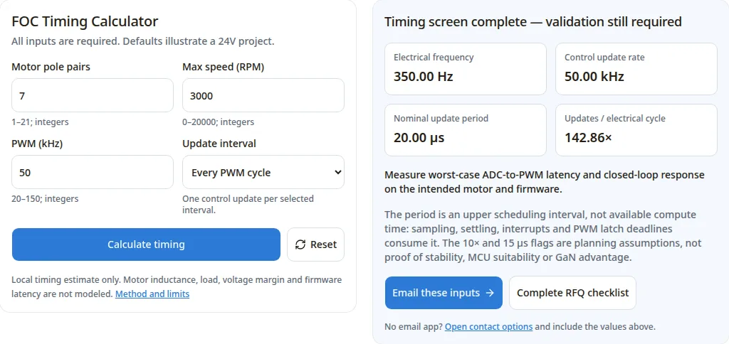
Figure 2: Existing software example from the 24V FOC timing tool, inspected November 1, 2026. Inputs of 7 pole pairs, 3,000 RPM, 50 kHz PWM and one update per cycle produce 350 Hz electrical frequency and a 20 µs nominal update period. It does not demonstrate 100 kHz–200 kHz hardware performance, sensor recovery, or measured loop stability.
Isolation can support a system insulation strategy, but barrier capacitance still couples switching transients. Differential magnetic sensing may reduce external-field error; test the mounted board near motor magnets, bus conductors, and cables. Do not call conductor losses negligible: an assumed 0.85 mΩ path dissipates 20² × 0.00085 = 0.34 W per phase, while other package resistances give different results.
Delay matters at the frequency being analyzed, not automatically at the PWM carrier. For an assumed pure delay of 400 ns, phase lag = 360° × frequency × delay: 1.44° at 10 kHz and 14.4° at 100 kHz. Include the sensor's frequency response, ADC, computation, and PWM update delay when assessing loop crossover. A 400 kHz sensor bandwidth alone neither rules out nor validates 100 kHz PWM.
Need a supplier review? Send the engineering team your bus extremes, RMS/peak phase currents, PWM strategy, and allowed current error to define the evidence required for a candidate design.
8. Supplier RFQ Checklist: Eight Technical Verifications
Use these requests to compare supplier evidence under the same conditions. Numerical examples above are screening assumptions, not universal acceptance thresholds.
- 1. Topology and sampling states: Obtain shunt/sensor locations, channel count, PWM sectors, maximum phase duties, contiguous sampling windows, and reconstruction or pulse-shifting policy at both intended PWM frequencies.
- 2. Common-mode range and transient recovery: Request measured input voltage, rise/fall rates, undershoot, and residual amplifier error at the ADC instant. Compare them with the exact datasheet test conditions; do not substitute AC CMRR for an edge-rate test.
- 3. End-to-end timing and accuracy: Define the allowable current error, acquisition time, common-mode recovery, filtering and latency across gain, load and temperature. Treat a sub-500 ns recovery target as a project requirement only if the system budget needs it and the candidate can demonstrate it.
- 4. Shunt/conductor thermal evidence: Request RMS and peak waveforms, pulse duration, resistance tolerance, TCR, power derating and mounted temperature. Use the complete error budget; 50 ppm/°C alone permits 0.4% drift over 80°C.
- 5. Layout and mounted interference: Review Kelvin pickup, input filter matching, return paths, clearance and nearby magnetic fields. Ask for waveforms on the intended layout, motor and cable assembly.
- 6. Hardware overcurrent shutdown: Obtain fault-current rise, threshold/blanking, worst-case sensor/comparator and driver delays, and the actual GaN device's protection limits. Require an autonomous shutdown path where needed; neither a 400 ns target nor an IC fault pin proves safe gate-off.
- 7. Control rates and loop response: Record PWM, ADC and FOC update rates separately, including decimation and worst-case execution time. Request measured closed-loop response and phase/gain margin at the intended operating points.
- 8. Trigger jitter and release criteria: Request ADC trigger timing relative to both PWM edges, jitter, and PWM latch deadline. Convert jitter to current error using the measured current slope; define acceptance limits, firmware version, temperature and retest conditions.
9. Frequently Asked Questions
Can a single DC-link shunt work at 100 kHz?
It can, if the PWM sequence provides the required active-vector sampling intervals and the full acquisition chain fits. The challenge is obtaining enough valid samples to reconstruct phase currents across sectors, particularly near short vectors. Request the usable modulation map and measured error; frequency alone cannot establish feasibility or rejection.
Does in-line current sensing prevent bearing currents?
No. Bearing-current risk involves common-mode voltage, motor and cable capacitances, bearings, chassis, and return paths. An in-line shunt does not remove those paths or prove EMC compliance. Its transient measurement error and the motor's bearing-current mitigation need separate validation.
What current-loop bandwidth is guaranteed by 100 kHz PWM?
None. A sample-rate-to-crossover ratio around 10:1 can be an initial design screen, not a stability guarantee. Establish the actual sample/update rates, total delay, motor model, controller tuning and measured loop response. A decimated update rate may meet the application's bandwidth requirement; verify rather than reject it automatically.
Can reconstruction compensate for low-side sampling limitations?
Sometimes. Sampling another phase pair, changing pulse timing, or estimating missing samples can extend coverage. These methods have operating limits and may alter ripple or noise. Compare measured current error, torque ripple and acoustic behavior at the required speed/load before selecting an architecture.
How should negative phase-node undershoot be specified?
Measure amplitude and duration at the sense inputs, including dead-time and parasitic ringing. Compare both recommended operating and absolute maximum ratings: survival does not establish accurate output. INA240 lists −4V operation and INA241x lists −5V operation; actual filter and layout behavior still require verification.
10. Procurement and Engineering Action Plan
- Define the operating envelope: Minimum/maximum bus voltage including charging and regeneration, phase RMS/peak current and pulse duration, motor inductance, PWM frequency, required duty range, and target current error/bandwidth.
- Screen timing and error: Apply the window model to actual switching states and calculate shunt or conductor loss. Reject unsupported margins; retain unknown values as supplier questions.
- Request matched evidence: Compare candidate waveforms at the same bus, motor, cable, temperature, gain and firmware conditions, including transient recovery and complete fault-to-gate-off timing.
- Approve against project limits: Complete thermal, EMC, insulation and protection validation separately. These calculations and a supplier datasheet do not establish certification or production approval.
For an OEM design discussion, review the 24V servo module planning guide and custom motor-control PCBA resource. Contact GAN Servo with your operating envelope and the checklist above to define a design review and evaluation plan.
Sources & References
Official sources checked November 1, 2026. Recheck the current revision and exact ordering code before design release:
- Texas Instruments — INA240 datasheet, Rev. C. Front page and sections 7–9 support the common-mode range, AC CMRR, PWM-rejection behavior and application limits. They do not qualify a complete 200 kHz inverter.
- Texas Instruments — INA241x datasheet, Rev. D. Front page and electrical characteristics distinguish bandwidth, settling and the stated switching-frequency support up to 125 kHz.
- Analog Devices / Maxim — MAX40056F/MAX40056T/MAX40056U datasheet, Rev. 8. Front page specifies PWM-edge recovery under the stated 500 V/µs condition; do not reinterpret the units as V/ns.
- Allegro MicroSystems — ACS37002 product page. Top Features supports the bandwidth and maximum overcurrent-detection response quoted here. Conductor resistance and insulation selection remain package-specific.
Source boundary: The 1.025 µs acquisition budget, 2 pF coupling capacitance, shunt heating/drift and pure-delay calculations are illustrative engineering models. No linked source or screenshot is presented as a GAN Servo hardware test or customer result. Revisit this guide within 12 months, or sooner if a cited device revision changes the selection limits.
Author

Categories
More Posts
48V GaN Servo Architecture for Humanoid and AMR Procurement
See why 48V GaN servo drives help humanoid and AMR teams cut harness weight, manage heat, vet suppliers, and request a 48V evaluation kit for pilot sourcing.

Regenerative Braking and DC-Bus Overvoltage in 48V GaN Servo Drives: Sizing Brake Choppers, Zero-Avalanche Protection, and Robotics Sourcing
Size brake choppers for 48V GaN servo drives, assess bus overvoltage and BMS disconnect risks, and request evidence with a seven-point supplier RFQ checklist.
Dual-Absolute Encoders in GaN Servo Actuators: Motor vs. Joint-Side Feedback, Mitigating 50V/ns dv/dt on BiSS-C/SSI, Harmonic Compliance, and Robotics Sourcing
Compare dual-absolute encoders in GaN servo actuators: BiSS-C/SSI noise, motor vs. joint feedback, gear compliance, and an RFQ checklist. Plan your review.